Exploring Lorentz Transformation with Mathematica: A Guide for Digital Nomads, Programmers, and Scientists

Relativity theory is one of the most fascinating and fundamental concepts in modern physics. At its core lies the Lorentz transformation, a set of equations that describe how measurements of space and time change for observers in different inertial frames. For digital nomads, programmers, and data scientists, understanding these concepts and leveraging tools like Mathematica can offer deep insights and powerful computational capabilities. This article delves into the Lorentz transformation, explores its role in relativity theory, and demonstrates how to use Mathematica to visualize and calculate these transformations.

Introduction to Relativity Theory

What is Relativity Theory?

Relativity theory, formulated by Albert Einstein, comprises two theories: Special Relativity and General Relativity. Special Relativity focuses on the physics of objects moving at constant speeds, particularly those close to the speed of light. General Relativity extends these concepts to include gravity and acceleration.

Importance of Lorentz Transformation

The Lorentz transformation is critical in Special Relativity, providing the mathematical framework to understand how different observers perceive space and time. It reconciles the constancy of the speed of light with the principle of relativity, which states that the laws of physics are the same for all non-accelerating observers.

Understanding Lorentz Transformation

The Equations

The Lorentz transformation equations relate the space and time coordinates of one inertial frame to another moving at a constant velocity relative to the first. The equations are:

$$ x' = \gamma (x - vt) \\
t' = \gamma \left(t - \frac{vx}{c^2}\right) \\
y' = y \\
z' = z $$

where:

$x, y, z, t $ are the coordinates in the original frame.
$x', y', z', t' $ are the coordinates in the moving frame.
$v $ is the relative velocity between the frames.
$c $ is the speed of light.
$\gamma $ (the Lorentz factor) is given by $$ \gamma = \frac{1}{\sqrt{1 - \frac{v^2}{c^2}}} $$.

Significance of the Lorentz Factor

The Lorentz factor $\gamma $ increases with velocity and approaches infinity as $v $ approaches the speed of light. This factor explains phenomena like time dilation (moving clocks run slower) and length contraction (moving objects appear shorter).

Using Mathematica to Explore Lorentz Transformation

Why Mathematica?

Mathematica is a powerful computational tool that allows for symbolic computation, numerical analysis, and visualization. It's particularly useful for digital nomads, programmers, and data scientists who need to perform complex calculations and create dynamic visualizations.

Setting Up Mathematica

Ensure you have Mathematica installed on your system. If you don't have it, download and install it from the official website. Familiarize yourself with the basic commands and interface.

Example 1: Visualizing Lorentz Transformation

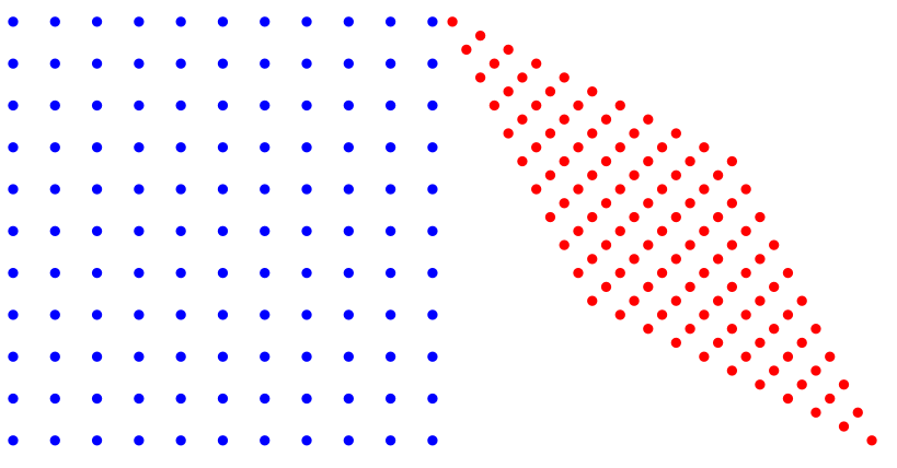
Let's start by visualizing the Lorentz transformation. We'll create a simple animation to show how the coordinates change under a Lorentz transformation.

Mathematica Code

(* Define parameters *)

v = 0.5; (* velocity as a fraction of the speed of light *)

c = 1; (* speed of light *)

gamma = 1/Sqrt[1 - v^2/c^2];

(* Define Lorentz transformation functions *)

lorentzX[x_, t_] := gamma (x - v t);

lorentzT[x_, t_] := gamma (t - (v x)/c^2);

(* Create a grid of points *)

points = Table[{x, t}, {x, -5, 5, 1}, {t, -5, 5, 1}];

transformedPoints = Table[{lorentzX[x, t], lorentzT[x, t]}, {x, -5, 5, 1}, {t, -5, 5, 1}];

(* Visualize the original and transformed grids *)

originalGrid = Graphics[{PointSize[Large], Blue, Point /@ Flatten[points, 1]}];

transformedGrid = Graphics[{PointSize[Large], Red, Point /@ Flatten[transformedPoints, 1]}];

(* Show the grids side by side *)

GraphicsGrid[{{originalGrid, transformedGrid}}, Spacings -> {2, 0}]

Output

This code will generate two grids: one representing the original coordinates and one representing the transformed coordinates. The visualization helps you see how points in space and time are shifted under the Lorentz transformation.

Example 2: Calculating Time Dilation

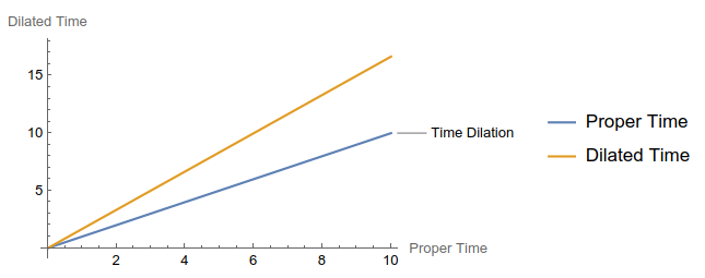
Time dilation is one of the most intriguing consequences of the Lorentz transformation. It predicts that a clock moving relative to an observer will tick slower than a clock at rest with respect to the observer.

Mathematica Code

(* Define parameters *)

v = 0.8; (* velocity as a fraction of the speed of light *)

c = 1; (* speed of light *)

gamma = 1/Sqrt[1 - v^2/c^2];

(* Define proper time and dilated time functions *)

properTime[t_] := t;

dilatedTime[t_] := gamma t;

(* Plot proper time vs. dilated time *)

timePlot = Plot[{properTime[t], dilatedTime[t]}, {t, 0, 10},

PlotLegends -> {"Proper Time", "Dilated Time"},

PlotLabels -> {"Time Dilation"},

AxesLabel -> {"Proper Time", "Dilated Time"}];

timePlot

Output

This plot shows the proper time (time measured by a stationary observer) and the dilated time (time measured by a moving observer). The dilated time increases more slowly than the proper time, illustrating time dilation.

Example 3: Length Contraction

Length contraction is another consequence of the Lorentz transformation, predicting that objects moving relative to an observer appear shorter along the direction of motion.

Mathematica Code

(* Define parameters *)

v = 0.8; (* velocity as a fraction of the speed of light *)

c = 1; (* speed of light *)

gamma = 1/Sqrt[1 - v^2/c^2];

(* Define proper length and contracted length functions *)

properLength[L_] := L;

contractedLength[L_] := L/gamma;

(* Plot proper length vs. contracted length *)

lengthPlot = Plot[{properLength[L], contractedLength[L]}, {L, 0, 10},

PlotLegends -> {"Proper Length", "Contracted Length"},

PlotLabels -> {"Length Contraction"},

AxesLabel -> {"Proper Length", "Contracted Length"}];

lengthPlot

Output

This plot compares the proper length (length measured by a stationary observer) and the contracted length (length measured by a moving observer). The contracted length is shorter, demonstrating length contraction.

Practical Applications

Relativity in Modern Technology

Relativity theory, particularly the Lorentz transformation, has practical applications in modern technology. For example, GPS systems must account for time dilation to provide accurate positioning data.

Conclusion

The Lorentz transformation is a cornerstone of relativity theory, providing critical insights into how space and time are interconnected. Whether you're calculating time dilation, visualizing transformations, or modeling relativistic effects, Mathematica offers the tools you need to deepen your understanding and enhance your work in relativity theory and universe. Happy exploring!