Feynman Path Integral: An Introduction with Mathematica Visualization

The Feynman path integral formulation is a cornerstone of quantum mechanics, providing an alternative to the traditional wave function approach. It was developed by Richard Feynman in the 1940s and has since become an essential tool in theoretical physics. This formulation describes the behavior of particles by considering all possible paths they can take and summing their contributions.

Introduction to Feynman Path Integral

The Feynman path integral formulation states that the probability amplitude for a particle to move from point \(A \) to point \(B \) is given by summing over all possible paths that the particle can take between these points. Each path is assigned a phase factor \( e^{iS/\hbar} \), where \(S \) is the classical action along the path.

Mathematically, the path integral is written as:

$$ \langle B | e^{-iHt/\hbar} | A \rangle = \int \mathcal{D}[x(t) e^{iS[x(t)]/\hbar} ] $$

where:

• \(\langle B | e^{-iHt/\hbar} | A \rangle \) is the propagator, representing the probability amplitude.
• \(\mathcal{D}[x(t)] \) denotes the integration over all possible paths \(x(t) \) from \(x(0) = A \) to \(x(t)=B \).
• \(S[x(t)] \) is the action for the path \(x(t) \).

Visualization of the Path Integral in Mathematica

Let's visualize the concept of Feynman path integrals using Mathematica. We'll consider a simple quantum mechanical system: a free particle moving in one dimension.

Setting Up the Problem

First, let's define the classical action for a free particle, which is given by:

$$ S = \int_{t_0}^{t_1} \frac{1}{2} m \left( \frac{dx}{dt} \right)^2 dt $$

where \(m \) the mass of the particle.

Mathematica Code for Path Integral Visualization

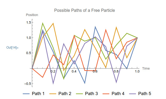
Below is the Mathematica code to visualize several possible paths a particle can take from point \(A \) to point \(B \) over a given time interval. We'll then compute the action for each path and illustrate the phase factors.

Explanation of the Code

1. Parameters: We define the mass of the particle, initial and final times, and initial and final positions. We also specify the number of paths to visualize.
2. Random Paths: We generate several random paths between points \(A \) and \(B \) using the RandomReal function.
3. Time Points: We define the time points at which the positions are sampled.
4. Action Calculation: We compute the classical action for each path using the definition of action for a free particle.
5. Phase Factors: We compute the phase factors \(e^{iS/\hbar} \) for each path.
6. Plotting Paths: We use ListLinePlot to plot the random paths and Show to display all the paths on a single plot.

Interpretation

The plot generated by the code shows several possible paths a particle can take from point \(A \) to point \(B \). Each path contributes to the overall probability amplitude with a phase factor determined by its action. In a real quantum mechanical system, an infinite number of such paths would be considered, and their contributions would be summed to determine the particle's behavior.

Conclusion

The Feynman path integral formulation provides a powerful framework for understanding quantum mechanics. By considering all possible paths and summing their contributions, it offers a deep insight into the probabilistic nature of quantum systems. Using Mathematica, we can visualize these concepts and gain a better understanding of the underlying principles of quantum mechanics.